


What is a Time Series?
In mathematics, a time series is a series of data points indexed (or listed or graphed) in time order. Most commonly, a time series is a sequence taken at successive equally spaced points in time. Thus it is a sequence of discrete-time data. Examples of time series are heights of ocean tides, counts of sunspots, and the daily closing value of the Dow Jones Industrial Average. Wikipedia.com
 Time series: random data plus trend, with best-fit line and different applied filters
What are seasonal effects?
A seasonal effect is a systematic and calendar related effect. Some examples include the sharp escalation in most Retail series which occurs around December in response to the Christmas period, or an increase in water consumption in summer due to warmer weather. Other seasonal effects include trading day effects (the number of working or trading days in a given month differs from year to year which will impact upon the level of activity in that month) and moving holiday (the timing of holidays such as Easter varies, so the effects of the holiday will be experienced in different periods each year). Australia Bureau of Statistics
What is Seasonality?
 The seasonal component consists of effects that are reasonably stable with respect to timing, direction and magnitude. It arises from systematic, calendar related influences such as:
- Natural Conditions weather fluctuations that are representative of the season (uncharacteristic weather patterns such as snow in summer would be considered irregular influences)
- Business and Administrative procedures start and end of the school term
- Social and Cultural behaviour
Australia Bureau of Statistics
Let's write some code
conda install numpy cython -c conda-forge
conda install matplotlib scipy pandas -c conda-forge
conda install pystan -c conda-forge
conda install -c anaconda ephem
pip install sklearn
pip install jupyter
pip install statsmodels --upgrade --user
conda install -c conda-forge fbpropeht
conda install -c conda-forge prophet
Let's import some libraries
import pandas as pd
import datetime as dt
import numpy as np
import matplotlib.pyplot as plt
import matplotlib.dates as mdates
Import the dataset (You can download the dataset from AirPassengers.csv)
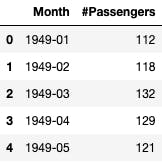
dt=pd.read_csv('AirPassengers.csv')
Let's take a look at the DataFrame
dt.head()
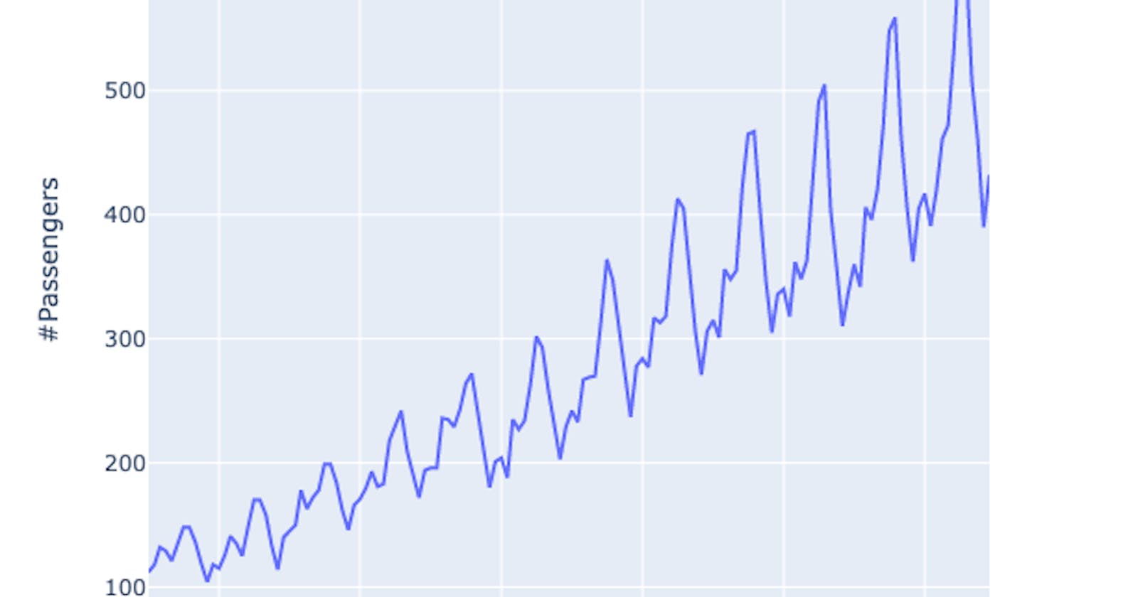
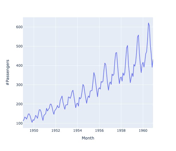
Plot the trend line
fig = px.line(dt,x='Month', y='#Passengers')
fig
Rename our columns and reformat our "x" column
dt['Month']=pd.to_datetime(dt['Month'], format='%Y-%m')
dt.rename(columns={'Month':'ds','#Passengers':'y'},inplace=True)
ADF test
In statistics and econometrics, an augmented Dickey–Fuller test (ADF) tests the null hypothesis that a unit root is present in a time series sample. The alternative hypothesis is different depending on which version of the test is used, but is usually stationarity or trend-stationarity. It is an augmented version of the Dickey–Fuller test for a larger and more complicated set of time series models. Wikipedia
from statsmodels.tsa.stattools import adfuller
dftest = adfuller(dt.y, autolag='AIC')
print("Test statistic = {:.3f}".format(dftest[0]))
print("P-value = {:.3f}".format(dftest[1]))
print("Critical values :")
for k, v in dftest[4].items():
    print("\t{}: {} - The data is {} stationary with {}% confidence".format(k, v, "not" if v<dftest[0] else "", 100-int(k[:-1])))
Test statistic = 0.815
P-value = 0.992
Critical values :
    1%: -3.4816817173418295 - The data is not stationary with 99% confidence
    5%: -2.8840418343195267 - The data is not stationary with 95% confidence
    10%: -2.578770059171598 - The data is not stationary with 90% confidence
P-value: the probability that a particular statistical measure, such as the mean or standard deviation, of an assumed probability distribution will be greater than or equal to (or less than or equal to in some instances) observed results.
AIC: In statistics, AIC is used to compare different possible models and determine which one is the best fit for the data. AIC is calculated from: the number of independent variables used to build the model. the maximum likelihood estimate of the model (how well the model reproduces the data).
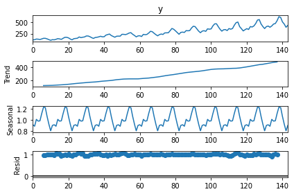
Time series decomposition
from statsmodels.tsa.seasonal import seasonal_decompose
result=seasonal_decompose(dt['y'], model='multiplicative', period=12)
result.plot()
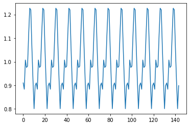
Season
result.seasonal.plot()
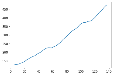
 Trend
Trend
result.trend.plot()
Divide train and test set for predictions
df = pd.DataFrame(dt, columns=['ds','y']).set_index('ds')
train = dt.iloc[:-12, :]
test = dt.iloc[-12:, :]
train.index = train.index
test.index = test.index
pred = test.copy()
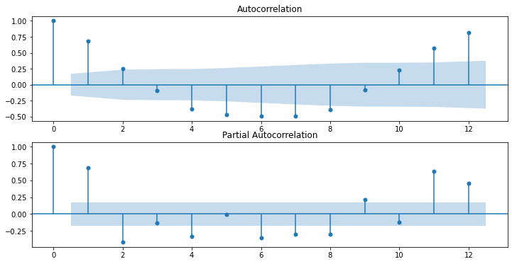
ACF and PACF Plots
ACF
ACF is an (complete) auto-correlation function which gives us values of auto-correlation of any series with its lagged values. We plot these values along with the confidence band and tada! We have an ACF plot. In simple terms, it describes how well the present value of the series is related with its past values. A time series can have components like trend, seasonality, cyclic and residual. ACF considers all these components while finding correlations hence it’s a ‘complete auto-correlation plot’.
PACF
PACF is a partial auto-correlation function. Basically instead of finding correlations of present with lags like ACF, it finds correlation of the residuals (which remains after removing the effects which are already explained by the earlier lag(s)) with the next lag value hence ‘partial’ and not ‘complete’ as we remove already found variations before we find the next correlation. So if there is any hidden information in the residual which can be modeled by the next lag, we might get a good correlation and we will keep that next lag as a feature while modeling. Remember while modeling we don’t want to keep too many features which are correlated as that can create multicollinearity issues. Hence we need to retain only the relevant features. Jayesh Salvi
from statsmodels.graphics.tsaplots import plot_acf, plot_pacf

dt['z_data'] = (dt['y'] - dt.y.rolling(window=12).mean()) / dt.y.rolling(window=12).std()

fig, ax = plt.subplots(2, figsize=(12,6))
ax[0] = plot_acf(dt.z_data.dropna(), ax=ax[0], lags=12)
ax[1] = plot_pacf(dt.z_data.dropna(), ax=ax[1], lags=12)
Smoothing
Smoothing refers to estimating a smooth trend, usually by means of weighted averages of observations. The term smooth is used because such averages tend to reduce randomness by allowing positive and negative random effects to partially offset each other. EUROSTAT
Simple
from statsmodels.tsa.holtwinters import SimpleExpSmoothing, Holt
model = SimpleExpSmoothing(np.asarray(train['y']))
3 models with different levels of smoothing
fit1 = model.fit()
pred1 = fit1.forecast(12)

fit2 = model.fit(smoothing_level=.2)
pred2 = fit2.forecast(12)

fit3 = model.fit(smoothing_level=.5)
pred3 = fit3.forecast(12)
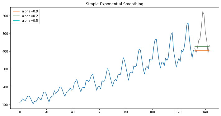 Note that this do not have trend or seasonality since Single Exponential Smoothing, SES for short, also called Simple Exponential Smoothing, is a time series forecasting method for univariate data without a trend or seasonality. It requires a single parameter, called alpha (a), also called the smoothing factor or smoothing coefficient.
Let's look at the formula
Using the naïve method, all forecasts for the future are equal to the last observed value of the series
 Using the average method, all future forecasts are equal to a simple average of the observed data,
 Forecasts are calculated using weighted averages, where the weights decrease exponentially as observations come from further in the past — the smallest weights are associated with the oldest observations:
 Rob J Hyndman and George Athanasopoulos
Holt Exponential Smoothing
model = Holt(np.asarray(train['y']))


fit1 = model.fit(smoothing_level=.3, smoothing_slope=.05)
pred1 = fit1.forecast(12)
fit2 = model.fit(optimized=True)
pred2 = fit2.forecast(12)
fit3 = model.fit(smoothing_level=.3, smoothing_slope=.02)
pred3 = fit3.forecast(12)

fig, ax = plt.subplots(figsize=(12, 6))
ax.plot(train.index, train.y.values)
ax.plot(test.index, test.y.values, color="gray")
for p, f, c in zip((pred1, pred2, pred3),(fit1, fit2, fit3),('#ff7823','#3c763d','c')):
    ax.plot(test.index, p, label="alpha="+str(f.params['smoothing_level'])[:3], color=c)
plt.title("Holt Exponential Smoothing")
plt.legend();
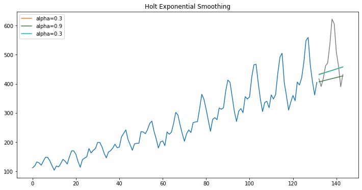
Holt’s Smoothing method: Holt’s smoothing technique, also known as linear exponential smoothing, is a widely known smoothing model for forecasting data that has a trend.
Holt (1957) extended simple exponential smoothing to allow the forecasting of data with a trend. This method involves a forecast equation and two smoothing equations (one for the level and one for the trend):
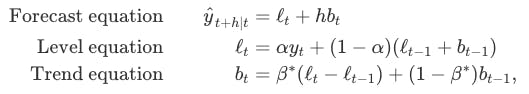 Rob J Hyndman and George Athanasopoulos
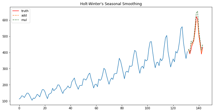
Holt- Winters
Holt-Winters is a model of time series behavior. Forecasting always requires a model, and Holt-Winters is a way to model three aspects of the time series: a typical value (average), a slope (trend) over time, and a cyclical repeating pattern (seasonality).
from statsmodels.tsa.holtwinters import ExponentialSmoothing
model = ExponentialSmoothing(np.asarray(train['y']), trend="add", seasonal="add", seasonal_periods=12)
model2 = ExponentialSmoothing(np.asarray(train['y']), trend="mul", seasonal="mul", seasonal_periods=12, damped=True)
fit = model.fit()
pred = fit.forecast(12)
fit2 = model2.fit()
pred2 = fit2.forecast(12)
fig, ax = plt.subplots(figsize=(12, 6))
ax.plot(train.index, train.y.values);
ax.plot(test.index, test.y.values, label='truth', color='red');
ax.plot(test.index, pred, linestyle='--', color='#ff7823', label='add');
ax.plot(test.index, pred2, linestyle='--', color='#3c763d',label='mul');
ax.legend();
ax.set_title("Holt-Winter's Seasonal Smoothing");

Charles C. Holt (21 May 1921 – 13 December 2010) was Professor at the Department of Management at the McCombs School of Business at the University of Texas at Austin. He is well known for his contributions (and for the contributions of his student, Peter Winters) to exponential smoothing
ARIMA
An ARIMA model is a class of statistical models for analyzing and forecasting time series data. It explicitly caters to a suite of standard structures in time series data, and as such provides a simple yet powerful method for making skillful time series forecasts.
- AR: Autoregression. A model that uses the dependent relationship between an observation and some number of lagged observations.
- I: Integrated. The use of differencing of raw observations (e.g. subtracting an observation from an observation at the previous time step) in order to make the time series stationary.
- MA: Moving Average. A model that uses the dependency between an observation and a residual error from a moving average model applied to lagged observations.
Parameters
- p: The number of lag observations included in the model, also called the lag order.
- d: The number of times that the raw observations are differenced, also called the degree of differencing.
- q: The size of the moving average window, also called the order of moving average.
from statsmodels.tsa.arima.model import ARIMA
from statsmodels.tsa.statespace.sarimax import SARIMAX
model = ARIMA(np.asarray(train['y']), order=(2,1,2))
model = SARIMAX(np.asarray(train['y']), order=(2,1,2), seasonal_order=(2,1,2,12))
model_fit = model.fit()
print(model_fit.summary())
RUNNING THE L-BFGS-B CODE

           * * *

Machine precision = 2.220D-16
 N =            9     M =           10

At X0         0 variables are exactly at the bounds

At iterate    0    f=  3.39336D+00    |proj g|=  1.30867D-01

At iterate    5    f=  3.37608D+00    |proj g|=  3.04657D-02
 This problem is unconstrained.

At iterate   10    f=  3.35722D+00    |proj g|=  2.69588D-02

At iterate   15    f=  3.34480D+00    |proj g|=  7.28348D-03

At iterate   20    f=  3.34111D+00    |proj g|=  4.29147D-04

 Bad direction in the line search;
   refresh the lbfgs memory and restart the iteration.

At iterate   25    f=  3.34110D+00    |proj g|=  9.72715D-04

 Bad direction in the line search;
   refresh the lbfgs memory and restart the iteration.

           * * *

Tit   = total number of iterations
Tnf   = total number of function evaluations
Tnint = total number of segments explored during Cauchy searches
Skip  = number of BFGS updates skipped
Nact  = number of active bounds at final generalized Cauchy point
Projg = norm of the final projected gradient
F     = final function value

           * * *

   N    Tit     Tnf  Tnint  Skip  Nact     Projg        F
    9     30     96      3     0     0   1.299D-03   3.341D+00
  F =   3.3411028337685020

ABNORMAL_TERMINATION_IN_LNSRCH
                                     SARIMAX Results
==========================================================================================
Dep. Variable:                                  y   No. Observations:                  132
Model:             SARIMAX(2, 1, 2)x(2, 1, 2, 12)   Log Likelihood                -441.026
Date:                            Fri, 18 Mar 2022   AIC                            900.051
Time:                                    00:10:33   BIC                            925.063
Sample:                                         0   HQIC                           910.208
                                            - 132
Covariance Type:                              opg
==============================================================================
                 coef    std err          z      P>|z|      [0.025      0.975]
------------------------------------------------------------------------------
ar.L1          0.3511      0.333      1.054      0.292      -0.302       1.004
ar.L2          0.4623      0.283      1.631      0.103      -0.093       1.018
ma.L1         -0.7040      0.356     -1.980      0.048      -1.401      -0.007
ma.L2         -0.2706      0.355     -0.763      0.445      -0.965       0.424
ar.S.L12       0.0352      0.256      0.137      0.891      -0.466       0.537
ar.S.L24       0.9617      0.353      2.728      0.006       0.271       1.653
ma.S.L12      -0.0946      1.836     -0.052      0.959      -3.692       3.503
ma.S.L24      -0.8639      1.844     -0.468      0.639      -4.478       2.750
sigma2        86.6275    142.098      0.610      0.542    -191.880     365.135
===================================================================================
Ljung-Box (L1) (Q):                   0.01   Jarque-Bera (JB):                 0.92
Prob(Q):                              0.93   Prob(JB):                         0.63
Heteroskedasticity (H):               1.39   Skew:                            -0.12
Prob(H) (two-sided):                  0.30   Kurtosis:                         3.36
===================================================================================

Warnings:
[1] Covariance matrix calculated using the outer product of gradients (complex-step).
/Users/daibeal/opt/anaconda3/lib/python3.9/site-packages/statsmodels/base/model.py:566: ConvergenceWarning:

Maximum Likelihood optimization failed to converge. Check mle_retvals


 Line search cannot locate an adequate point after MAXLS
  function and gradient evaluations.
  Previous x, f and g restored.
 Possible causes: 1 error in function or gradient evaluation;
                  2 rounding error dominate computation.
predictions = list()
n_pred=len(np.asarray(test['y']))
history=[x for x in np.asarray(train['y'])]
for t in range(n_pred):
    model = model
    model_fit = model.fit()
    output = model_fit.forecast(n_pred)
    yhat = output[t]
    predictions.append(yhat)
    obs = np.asarray(test['y'])[t]
    history.append(obs)
    print('predicted=%f, expected=%f' % (yhat, obs))
RUNNING THE L-BFGS-B CODE

           * * *

Machine precision = 2.220D-16
 N =            9     M =           10

At X0         0 variables are exactly at the bounds

At iterate    0    f=  3.39336D+00    |proj g|=  1.30867D-01

At iterate    5    f=  3.37608D+00    |proj g|=  3.04657D-02
 This problem is unconstrained.

At iterate   10    f=  3.35722D+00    |proj g|=  2.69588D-02

At iterate   15    f=  3.34480D+00    |proj g|=  7.28348D-03

At iterate   20    f=  3.34111D+00    |proj g|=  4.29147D-04

 Bad direction in the line search;
   refresh the lbfgs memory and restart the iteration.

At iterate   25    f=  3.34110D+00    |proj g|=  9.72715D-04

 Bad direction in the line search;
   refresh the lbfgs memory and restart the iteration.
/Users/daibeal/opt/anaconda3/lib/python3.9/site-packages/statsmodels/base/model.py:566: ConvergenceWarning:

Maximum Likelihood optimization failed to converge. Check mle_retvals


 Line search cannot locate an adequate point after MAXLS
  function and gradient evaluations.
  Previous x, f and g restored.
 Possible causes: 1 error in function or gradient evaluation;
                  2 rounding error dominate computation.
 This problem is unconstrained.

           * * *

Tit   = total number of iterations
Tnf   = total number of function evaluations
Tnint = total number of segments explored during Cauchy searches
Skip  = number of BFGS updates skipped
Nact  = number of active bounds at final generalized Cauchy point
Projg = norm of the final projected gradient
F     = final function value

           * * *

   N    Tit     Tnf  Tnint  Skip  Nact     Projg        F
    9     30     96      3     0     0   1.299D-03   3.341D+00
  F =   3.3411028337685020

ABNORMAL_TERMINATION_IN_LNSRCH
predicted=418.644068, expected=417.000000
RUNNING THE L-BFGS-B CODE

           * * *

Machine precision = 2.220D-16
 N =            9     M =           10

At X0         0 variables are exactly at the bounds

At iterate    0    f=  3.39336D+00    |proj g|=  1.30867D-01

At iterate    5    f=  3.37608D+00    |proj g|=  3.04657D-02

At iterate   10    f=  3.35722D+00    |proj g|=  2.69588D-02

At iterate   15    f=  3.34480D+00    |proj g|=  7.28348D-03

At iterate   20    f=  3.34111D+00    |proj g|=  4.29147D-04

 Bad direction in the line search;
   refresh the lbfgs memory and restart the iteration.

At iterate   25    f=  3.34110D+00    |proj g|=  9.72715D-04

 Bad direction in the line search;
   refresh the lbfgs memory and restart the iteration.
/Users/daibeal/opt/anaconda3/lib/python3.9/site-packages/statsmodels/base/model.py:566: ConvergenceWarning:

Maximum Likelihood optimization failed to converge. Check mle_retvals


 Line search cannot locate an adequate point after MAXLS
  function and gradient evaluations.
  Previous x, f and g restored.
 Possible causes: 1 error in function or gradient evaluation;
                  2 rounding error dominate computation.
 This problem is unconstrained.

           * * *

Tit   = total number of iterations
Tnf   = total number of function evaluations
Tnint = total number of segments explored during Cauchy searches
Skip  = number of BFGS updates skipped
Nact  = number of active bounds at final generalized Cauchy point
Projg = norm of the final projected gradient
F     = final function value

           * * *

   N    Tit     Tnf  Tnint  Skip  Nact     Projg        F
    9     30     96      3     0     0   1.299D-03   3.341D+00
  F =   3.3411028337685020

ABNORMAL_TERMINATION_IN_LNSRCH
predicted=397.649625, expected=391.000000
RUNNING THE L-BFGS-B CODE

           * * *

Machine precision = 2.220D-16
 N =            9     M =           10

At X0         0 variables are exactly at the bounds

At iterate    0    f=  3.39336D+00    |proj g|=  1.30867D-01

At iterate    5    f=  3.37608D+00    |proj g|=  3.04657D-02

At iterate   10    f=  3.35722D+00    |proj g|=  2.69588D-02

At iterate   15    f=  3.34480D+00    |proj g|=  7.28348D-03

At iterate   20    f=  3.34111D+00    |proj g|=  4.29147D-04

 Bad direction in the line search;
   refresh the lbfgs memory and restart the iteration.

At iterate   25    f=  3.34110D+00    |proj g|=  9.72715D-04

 Bad direction in the line search;
   refresh the lbfgs memory and restart the iteration.
/Users/daibeal/opt/anaconda3/lib/python3.9/site-packages/statsmodels/base/model.py:566: ConvergenceWarning:

Maximum Likelihood optimization failed to converge. Check mle_retvals


 Line search cannot locate an adequate point after MAXLS
  function and gradient evaluations.
  Previous x, f and g restored.
 Possible causes: 1 error in function or gradient evaluation;
                  2 rounding error dominate computation.
 This problem is unconstrained.

           * * *

Tit   = total number of iterations
Tnf   = total number of function evaluations
Tnint = total number of segments explored during Cauchy searches
Skip  = number of BFGS updates skipped
Nact  = number of active bounds at final generalized Cauchy point
Projg = norm of the final projected gradient
F     = final function value

           * * *

   N    Tit     Tnf  Tnint  Skip  Nact     Projg        F
    9     30     96      3     0     0   1.299D-03   3.341D+00
  F =   3.3411028337685020

ABNORMAL_TERMINATION_IN_LNSRCH
predicted=456.597187, expected=419.000000
RUNNING THE L-BFGS-B CODE

           * * *

Machine precision = 2.220D-16
 N =            9     M =           10

At X0         0 variables are exactly at the bounds

At iterate    0    f=  3.39336D+00    |proj g|=  1.30867D-01

At iterate    5    f=  3.37608D+00    |proj g|=  3.04657D-02

At iterate   10    f=  3.35722D+00    |proj g|=  2.69588D-02

At iterate   15    f=  3.34480D+00    |proj g|=  7.28348D-03

At iterate   20    f=  3.34111D+00    |proj g|=  4.29147D-04

 Bad direction in the line search;
   refresh the lbfgs memory and restart the iteration.

At iterate   25    f=  3.34110D+00    |proj g|=  9.72715D-04

 Bad direction in the line search;
   refresh the lbfgs memory and restart the iteration.
/Users/daibeal/opt/anaconda3/lib/python3.9/site-packages/statsmodels/base/model.py:566: ConvergenceWarning:

Maximum Likelihood optimization failed to converge. Check mle_retvals


 Line search cannot locate an adequate point after MAXLS
  function and gradient evaluations.
  Previous x, f and g restored.
 Possible causes: 1 error in function or gradient evaluation;
                  2 rounding error dominate computation.
 This problem is unconstrained.

           * * *

Tit   = total number of iterations
Tnf   = total number of function evaluations
Tnint = total number of segments explored during Cauchy searches
Skip  = number of BFGS updates skipped
Nact  = number of active bounds at final generalized Cauchy point
Projg = norm of the final projected gradient
F     = final function value

           * * *

   N    Tit     Tnf  Tnint  Skip  Nact     Projg        F
    9     30     96      3     0     0   1.299D-03   3.341D+00
  F =   3.3411028337685020

ABNORMAL_TERMINATION_IN_LNSRCH
predicted=442.471865, expected=461.000000
RUNNING THE L-BFGS-B CODE

           * * *

Machine precision = 2.220D-16
 N =            9     M =           10

At X0         0 variables are exactly at the bounds

At iterate    0    f=  3.39336D+00    |proj g|=  1.30867D-01

At iterate    5    f=  3.37608D+00    |proj g|=  3.04657D-02

At iterate   10    f=  3.35722D+00    |proj g|=  2.69588D-02

At iterate   15    f=  3.34480D+00    |proj g|=  7.28348D-03

At iterate   20    f=  3.34111D+00    |proj g|=  4.29147D-04

 Bad direction in the line search;
   refresh the lbfgs memory and restart the iteration.

At iterate   25    f=  3.34110D+00    |proj g|=  9.72715D-04

 Bad direction in the line search;
   refresh the lbfgs memory and restart the iteration.
/Users/daibeal/opt/anaconda3/lib/python3.9/site-packages/statsmodels/base/model.py:566: ConvergenceWarning:

Maximum Likelihood optimization failed to converge. Check mle_retvals


 Line search cannot locate an adequate point after MAXLS
  function and gradient evaluations.
  Previous x, f and g restored.
 Possible causes: 1 error in function or gradient evaluation;
                  2 rounding error dominate computation.
 This problem is unconstrained.

           * * *

Tit   = total number of iterations
Tnf   = total number of function evaluations
Tnint = total number of segments explored during Cauchy searches
Skip  = number of BFGS updates skipped
Nact  = number of active bounds at final generalized Cauchy point
Projg = norm of the final projected gradient
F     = final function value

           * * *

   N    Tit     Tnf  Tnint  Skip  Nact     Projg        F
    9     30     96      3     0     0   1.299D-03   3.341D+00
  F =   3.3411028337685020

ABNORMAL_TERMINATION_IN_LNSRCH
predicted=466.408105, expected=472.000000
RUNNING THE L-BFGS-B CODE

           * * *

Machine precision = 2.220D-16
 N =            9     M =           10

At X0         0 variables are exactly at the bounds

At iterate    0    f=  3.39336D+00    |proj g|=  1.30867D-01

At iterate    5    f=  3.37608D+00    |proj g|=  3.04657D-02

At iterate   10    f=  3.35722D+00    |proj g|=  2.69588D-02

At iterate   15    f=  3.34480D+00    |proj g|=  7.28348D-03

At iterate   20    f=  3.34111D+00    |proj g|=  4.29147D-04

 Bad direction in the line search;
   refresh the lbfgs memory and restart the iteration.

At iterate   25    f=  3.34110D+00    |proj g|=  9.72715D-04

 Bad direction in the line search;
   refresh the lbfgs memory and restart the iteration.
/Users/daibeal/opt/anaconda3/lib/python3.9/site-packages/statsmodels/base/model.py:566: ConvergenceWarning:

Maximum Likelihood optimization failed to converge. Check mle_retvals


 Line search cannot locate an adequate point after MAXLS
  function and gradient evaluations.
  Previous x, f and g restored.
 Possible causes: 1 error in function or gradient evaluation;
                  2 rounding error dominate computation.
 This problem is unconstrained.

           * * *

Tit   = total number of iterations
Tnf   = total number of function evaluations
Tnint = total number of segments explored during Cauchy searches
Skip  = number of BFGS updates skipped
Nact  = number of active bounds at final generalized Cauchy point
Projg = norm of the final projected gradient
F     = final function value

           * * *

   N    Tit     Tnf  Tnint  Skip  Nact     Projg        F
    9     30     96      3     0     0   1.299D-03   3.341D+00
  F =   3.3411028337685020

ABNORMAL_TERMINATION_IN_LNSRCH
predicted=524.568310, expected=535.000000
RUNNING THE L-BFGS-B CODE

           * * *

Machine precision = 2.220D-16
 N =            9     M =           10

At X0         0 variables are exactly at the bounds

At iterate    0    f=  3.39336D+00    |proj g|=  1.30867D-01

At iterate    5    f=  3.37608D+00    |proj g|=  3.04657D-02

At iterate   10    f=  3.35722D+00    |proj g|=  2.69588D-02

At iterate   15    f=  3.34480D+00    |proj g|=  7.28348D-03

At iterate   20    f=  3.34111D+00    |proj g|=  4.29147D-04

 Bad direction in the line search;
   refresh the lbfgs memory and restart the iteration.

At iterate   25    f=  3.34110D+00    |proj g|=  9.72715D-04

 Bad direction in the line search;
   refresh the lbfgs memory and restart the iteration.

           * * *

Tit   = total number of iterations
Tnf   = total number of function evaluations
Tnint = total number of segments explored during Cauchy searches
Skip  = number of BFGS updates skipped
Nact  = number of active bounds at final generalized Cauchy point
Projg = norm of the final projected gradient
F     = final function value

           * * *

   N    Tit     Tnf  Tnint  Skip  Nact     Projg        F
    9     30     96      3     0     0   1.299D-03   3.341D+00
  F =   3.3411028337685020

ABNORMAL_TERMINATION_IN_LNSRCH
predicted=601.004765, expected=622.000000
RUNNING THE L-BFGS-B CODE

           * * *

Machine precision = 2.220D-16
 N =            9     M =           10

At X0         0 variables are exactly at the bounds

At iterate    0    f=  3.39336D+00    |proj g|=  1.30867D-01
/Users/daibeal/opt/anaconda3/lib/python3.9/site-packages/statsmodels/base/model.py:566: ConvergenceWarning:

Maximum Likelihood optimization failed to converge. Check mle_retvals


 Line search cannot locate an adequate point after MAXLS
  function and gradient evaluations.
  Previous x, f and g restored.
 Possible causes: 1 error in function or gradient evaluation;
                  2 rounding error dominate computation.
 This problem is unconstrained.

At iterate    5    f=  3.37608D+00    |proj g|=  3.04657D-02

At iterate   10    f=  3.35722D+00    |proj g|=  2.69588D-02

At iterate   15    f=  3.34480D+00    |proj g|=  7.28348D-03

At iterate   20    f=  3.34111D+00    |proj g|=  4.29147D-04

 Bad direction in the line search;
   refresh the lbfgs memory and restart the iteration.

At iterate   25    f=  3.34110D+00    |proj g|=  9.72715D-04

 Bad direction in the line search;
   refresh the lbfgs memory and restart the iteration.
/Users/daibeal/opt/anaconda3/lib/python3.9/site-packages/statsmodels/base/model.py:566: ConvergenceWarning:

Maximum Likelihood optimization failed to converge. Check mle_retvals


 Line search cannot locate an adequate point after MAXLS
  function and gradient evaluations.
  Previous x, f and g restored.
 Possible causes: 1 error in function or gradient evaluation;
                  2 rounding error dominate computation.
 This problem is unconstrained.

           * * *

Tit   = total number of iterations
Tnf   = total number of function evaluations
Tnint = total number of segments explored during Cauchy searches
Skip  = number of BFGS updates skipped
Nact  = number of active bounds at final generalized Cauchy point
Projg = norm of the final projected gradient
F     = final function value

           * * *

   N    Tit     Tnf  Tnint  Skip  Nact     Projg        F
    9     30     96      3     0     0   1.299D-03   3.341D+00
  F =   3.3411028337685020

ABNORMAL_TERMINATION_IN_LNSRCH
predicted=612.745350, expected=606.000000
RUNNING THE L-BFGS-B CODE

           * * *

Machine precision = 2.220D-16
 N =            9     M =           10

At X0         0 variables are exactly at the bounds

At iterate    0    f=  3.39336D+00    |proj g|=  1.30867D-01

At iterate    5    f=  3.37608D+00    |proj g|=  3.04657D-02

At iterate   10    f=  3.35722D+00    |proj g|=  2.69588D-02

At iterate   15    f=  3.34480D+00    |proj g|=  7.28348D-03

At iterate   20    f=  3.34111D+00    |proj g|=  4.29147D-04

 Bad direction in the line search;
   refresh the lbfgs memory and restart the iteration.

At iterate   25    f=  3.34110D+00    |proj g|=  9.72715D-04

 Bad direction in the line search;
   refresh the lbfgs memory and restart the iteration.
/Users/daibeal/opt/anaconda3/lib/python3.9/site-packages/statsmodels/base/model.py:566: ConvergenceWarning:

Maximum Likelihood optimization failed to converge. Check mle_retvals


 Line search cannot locate an adequate point after MAXLS
  function and gradient evaluations.
  Previous x, f and g restored.
 Possible causes: 1 error in function or gradient evaluation;
                  2 rounding error dominate computation.
 This problem is unconstrained.

           * * *

Tit   = total number of iterations
Tnf   = total number of function evaluations
Tnint = total number of segments explored during Cauchy searches
Skip  = number of BFGS updates skipped
Nact  = number of active bounds at final generalized Cauchy point
Projg = norm of the final projected gradient
F     = final function value

           * * *

   N    Tit     Tnf  Tnint  Skip  Nact     Projg        F
    9     30     96      3     0     0   1.299D-03   3.341D+00
  F =   3.3411028337685020

ABNORMAL_TERMINATION_IN_LNSRCH
predicted=506.346357, expected=508.000000
RUNNING THE L-BFGS-B CODE

           * * *

Machine precision = 2.220D-16
 N =            9     M =           10

At X0         0 variables are exactly at the bounds

At iterate    0    f=  3.39336D+00    |proj g|=  1.30867D-01

At iterate    5    f=  3.37608D+00    |proj g|=  3.04657D-02

At iterate   10    f=  3.35722D+00    |proj g|=  2.69588D-02

At iterate   15    f=  3.34480D+00    |proj g|=  7.28348D-03

At iterate   20    f=  3.34111D+00    |proj g|=  4.29147D-04

 Bad direction in the line search;
   refresh the lbfgs memory and restart the iteration.

At iterate   25    f=  3.34110D+00    |proj g|=  9.72715D-04

 Bad direction in the line search;
   refresh the lbfgs memory and restart the iteration.
/Users/daibeal/opt/anaconda3/lib/python3.9/site-packages/statsmodels/base/model.py:566: ConvergenceWarning:

Maximum Likelihood optimization failed to converge. Check mle_retvals


 Line search cannot locate an adequate point after MAXLS
  function and gradient evaluations.
  Previous x, f and g restored.
 Possible causes: 1 error in function or gradient evaluation;
                  2 rounding error dominate computation.
 This problem is unconstrained.

           * * *

Tit   = total number of iterations
Tnf   = total number of function evaluations
Tnint = total number of segments explored during Cauchy searches
Skip  = number of BFGS updates skipped
Nact  = number of active bounds at final generalized Cauchy point
Projg = norm of the final projected gradient
F     = final function value

           * * *

   N    Tit     Tnf  Tnint  Skip  Nact     Projg        F
    9     30     96      3     0     0   1.299D-03   3.341D+00
  F =   3.3411028337685020

ABNORMAL_TERMINATION_IN_LNSRCH
predicted=449.002229, expected=461.000000
RUNNING THE L-BFGS-B CODE

           * * *

Machine precision = 2.220D-16
 N =            9     M =           10

At X0         0 variables are exactly at the bounds

At iterate    0    f=  3.39336D+00    |proj g|=  1.30867D-01

At iterate    5    f=  3.37608D+00    |proj g|=  3.04657D-02

At iterate   10    f=  3.35722D+00    |proj g|=  2.69588D-02

At iterate   15    f=  3.34480D+00    |proj g|=  7.28348D-03

At iterate   20    f=  3.34111D+00    |proj g|=  4.29147D-04

 Bad direction in the line search;
   refresh the lbfgs memory and restart the iteration.

At iterate   25    f=  3.34110D+00    |proj g|=  9.72715D-04

 Bad direction in the line search;
   refresh the lbfgs memory and restart the iteration.
/Users/daibeal/opt/anaconda3/lib/python3.9/site-packages/statsmodels/base/model.py:566: ConvergenceWarning:

Maximum Likelihood optimization failed to converge. Check mle_retvals


 Line search cannot locate an adequate point after MAXLS
  function and gradient evaluations.
  Previous x, f and g restored.
 Possible causes: 1 error in function or gradient evaluation;
                  2 rounding error dominate computation.
 This problem is unconstrained.

           * * *

Tit   = total number of iterations
Tnf   = total number of function evaluations
Tnint = total number of segments explored during Cauchy searches
Skip  = number of BFGS updates skipped
Nact  = number of active bounds at final generalized Cauchy point
Projg = norm of the final projected gradient
F     = final function value

           * * *

   N    Tit     Tnf  Tnint  Skip  Nact     Projg        F
    9     30     96      3     0     0   1.299D-03   3.341D+00
  F =   3.3411028337685020

ABNORMAL_TERMINATION_IN_LNSRCH
predicted=401.928672, expected=390.000000
RUNNING THE L-BFGS-B CODE

           * * *

Machine precision = 2.220D-16
 N =            9     M =           10

At X0         0 variables are exactly at the bounds

At iterate    0    f=  3.39336D+00    |proj g|=  1.30867D-01

At iterate    5    f=  3.37608D+00    |proj g|=  3.04657D-02

At iterate   10    f=  3.35722D+00    |proj g|=  2.69588D-02

At iterate   15    f=  3.34480D+00    |proj g|=  7.28348D-03

At iterate   20    f=  3.34111D+00    |proj g|=  4.29147D-04

 Bad direction in the line search;
   refresh the lbfgs memory and restart the iteration.

At iterate   25    f=  3.34110D+00    |proj g|=  9.72715D-04

 Bad direction in the line search;
   refresh the lbfgs memory and restart the iteration.

           * * *

Tit   = total number of iterations
Tnf   = total number of function evaluations
Tnint = total number of segments explored during Cauchy searches
Skip  = number of BFGS updates skipped
Nact  = number of active bounds at final generalized Cauchy point
Projg = norm of the final projected gradient
F     = final function value

           * * *

   N    Tit     Tnf  Tnint  Skip  Nact     Projg        F
    9     30     96      3     0     0   1.299D-03   3.341D+00
  F =   3.3411028337685020

ABNORMAL_TERMINATION_IN_LNSRCH
predicted=444.344809, expected=432.000000
/Users/daibeal/opt/anaconda3/lib/python3.9/site-packages/statsmodels/base/model.py:566: ConvergenceWarning:

Maximum Likelihood optimization failed to converge. Check mle_retvals


 Line search cannot locate an adequate point after MAXLS
  function and gradient evaluations.
  Previous x, f and g restored.
 Possible causes: 1 error in function or gradient evaluation;
                  2 rounding error dominate computation.
fig, ax = plt.subplots(figsize=(12, 6))
ax.plot(train.index, train.y.values);
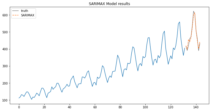
ax.plot(test.index, test.y.values, label='truth', color='grey');
ax.plot(test.index, predictions, linestyle='--', color='#ff7823', label='SARIMAX');
ax.legend();
ax.set_title("SARIMAX Model results");
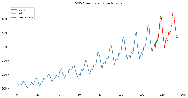
new_predictions=model_fit.forecast(24)
new_predictions
array([418.64406815, 397.64962523, 456.59718732, 442.47186484,
       466.40810521, 524.5683102 , 601.00476519, 612.74535017,
       506.34635712, 449.00222905, 401.92867198, 444.34480863,
       462.09793437, 439.54110638, 505.36873737, 492.23485772,
       517.52163824, 572.2595745 , 653.87078268, 664.65882656,
       556.61875719, 494.70124974, 444.77601598, 490.10593024])
t=range(132,156,1)
fig, ax = plt.subplots(figsize=(12, 6))

ax.plot(train.index, train.y.values);
ax.plot(test.index, test.y.values, label='truth', color='green');
ax.plot(test.index, predictions, linestyle='--', color='#ff7823', label='add');
ax.plot(t, new_predictions, linestyle='--', color='red', label='predicionts');

ax.legend();
ax.set_title("SARIMA results and predictions");
from sklearn.metrics import mean_squared_error

rms_sarima = mean_squared_error(test.y.values, predictions, squared=False)
rms_alisado = mean_squared_error(test.y.values, pred, squared=False)

Resultados= {
    'rms_sarima': rms_sarima,
    'rms_alisado':rms_alisado
}
print(Resultados)
{'rms_sarima': 15.469104677453062, 'rms_alisado': 16.980018018225735}
ARIMAX VS SARIMAX
The implementation is called SARIMAX instead of SARIMA because the “X” addition to the method name means that the implementation also supports exogenous variables. These are parallel time series variates that are not modeled directly via AR, I, or MA processes, but are made available as a weighted input to the model.
References
- Significance of ACF and PACF Plots In Time Series Analysis by Jayesh Salvi
- Smoothing by Eurostat
- Forecasting: Principles and Practice by Rob J Hyndman and George Athanasopoulos
- How to Create an ARIMA Model for Time Series Forecasting in Python by Jason Brownlee